Fast Surface Normal Generation

When one draws computer graphics the traditional way, using all of the rendering pipeline, it's easy to include surface orientation data right alongside other vertex data.

However when ray-marching one calculates geometry on the fly, and hence can't be buddied-up with pre-computed surface normals. How then does one calculate a surface normal?

After a while I thought to take the negative reciprocal of the local derivative (essentially a Sobel filtering) to create a vector that pointed out of the surface, and hence could be the surface normal. However, that takes a ton of sampling and division, both very time-heavy operations. Then I stumbled upon this gem.

/*
  Returns the surface normal of a point in the distance function.
*/
vec3 getNormal(vec3 pos)
{
  float d=getDist(pos);
  return normalize(vec3( getDist(pos+vec3(EPSILON,0,0))-d, getDist(pos+vec3(0,EPSILON,0))-d, getDist(pos+vec3(0,0,EPSILON))-d ));
}

Whoa, what is this mess? Let's refactor it for readability.

/*
  Returns the surface normal of a point in the distance function.
*/
vec3 getNormal(vec3 pos)
{
  float c=getDist(pos);
  vec3 n = vec3();
  n.x = getDist( pos+vec3(EPSILON,0,0) );
  n.y = getDist( pos+vec3(0,EPSILON,0) );
  n.z = getDist( pos+vec3(0,0,EPSILON) );
  n - c;
  return normalize(n);
}

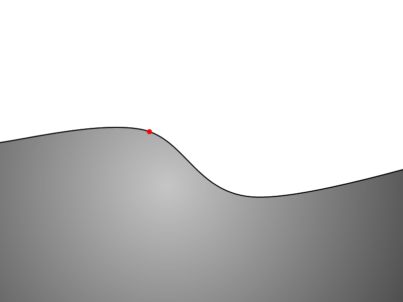
That's more expensive, but fathoms more pleasant to read. First, some clarification. This function relies on some predefined tokens. EPSILON is the maximum acceptable distance threshold, and getDist() is the distance function. Normalize() is a built-in to normalize a vector type. To understand what's going on here, let's step down into two dimensions and draw pictures. Here's a point that we've marched to the surface of a distance function.

The red dot is a point marched to the surface of a distance function.

Now remember that point does not exist exactly upon the surface, but rather has been marched to within a minimum distance (that we call epsilon) of the distance function. So if we zoom in by a great amount...

A close up of the prior figure.

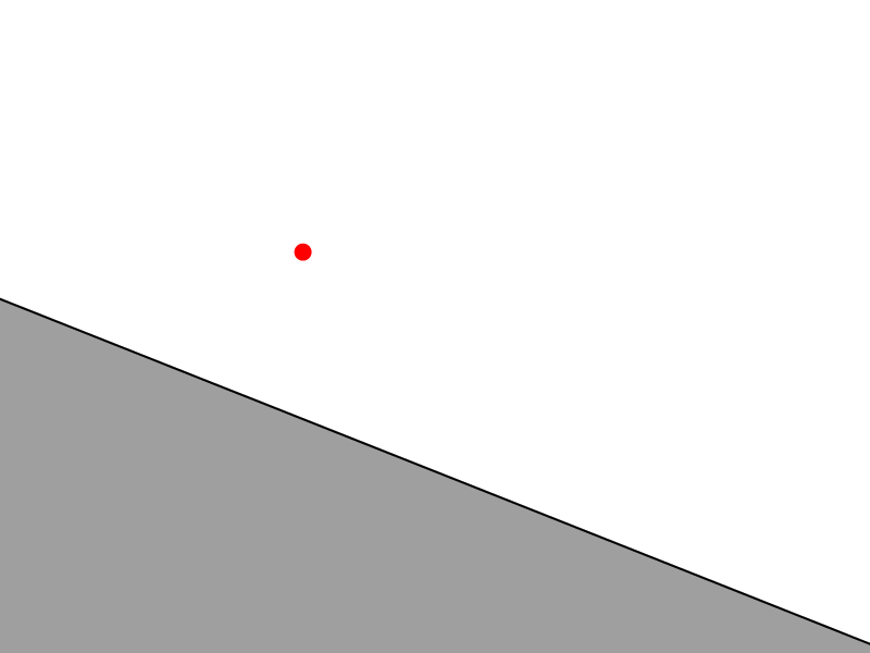
There are two important things to notice about this figure. First is the afore mentioned discontinuity in marched position versus actual position, and second, that at this scale nearly all surfaces approach linear gradients.

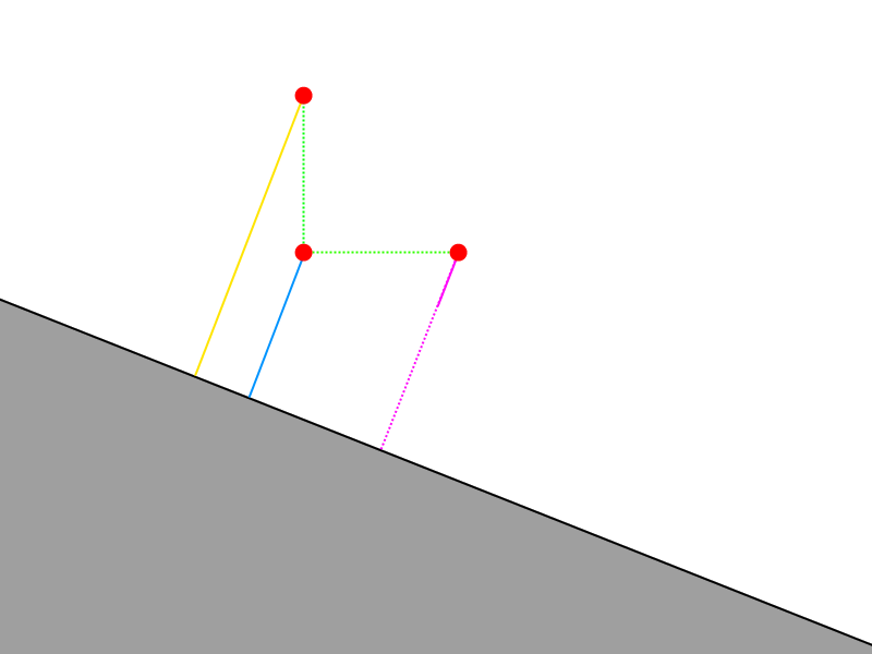
If we look at the function, we see that it samples the distance function epsilon away from the original point along the positive direction of each axis. Let's do that in our 2D illustration--first we do this along the X axis.

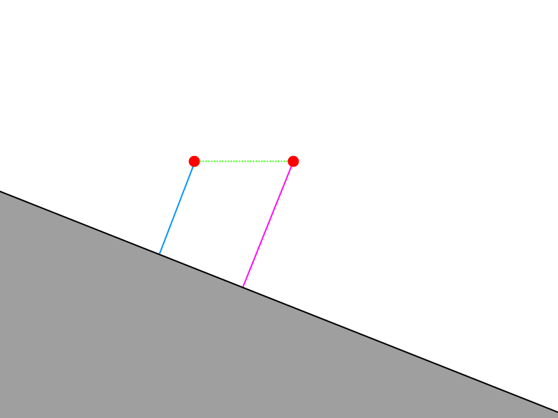
Sampling the distance function epsilon along the X axis. The new distance is represented by the purple line, with the original distance typified by the blue line, with the dotted green line being epsilon distance along the X axis.

Next we need to subtract the original distance from the value along the X axis. This will give us the magnitude of our normal vector in the X direction.

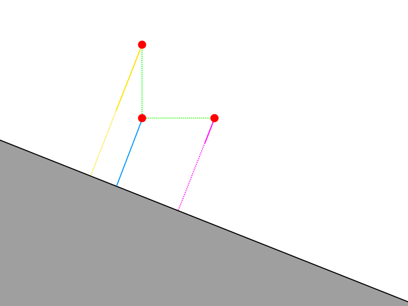
Subtracting the original distance from the freshly sampled distance. The subtracted portion is now dotted.

The next step is to sample the distance function epsilon along the Y axis away from the original point.

Sampling the distance function epsilon along the Y axis. This value is represented by the yellow line, with the translation epsilon along the Y axis drawn out in dotted green.

Again we subtract epsilon from this sampled distance, and this time we arrive at the magnitude of the Y component of our normal vector.

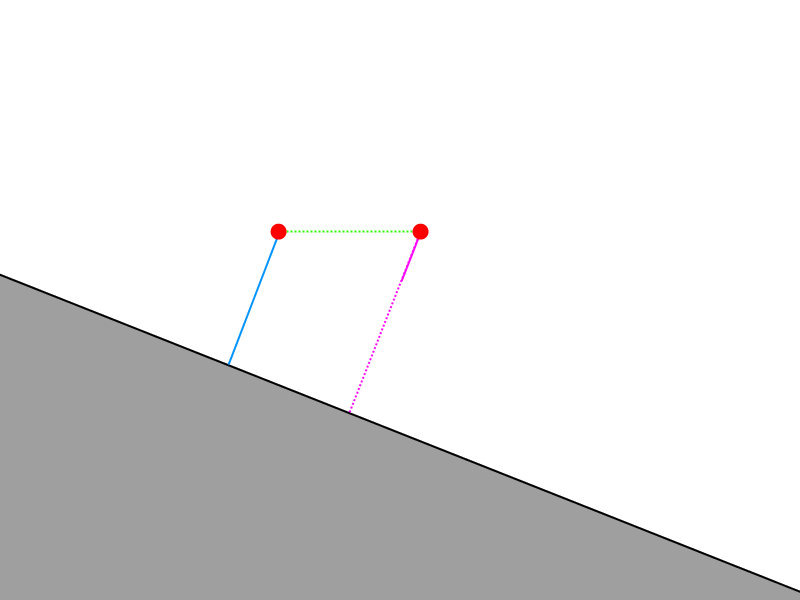
Subtracting the original distance. The dotted portion of the yellow line is the result of our work.

Now if we were to construct a vector using these terms, this is what we would arrive at.

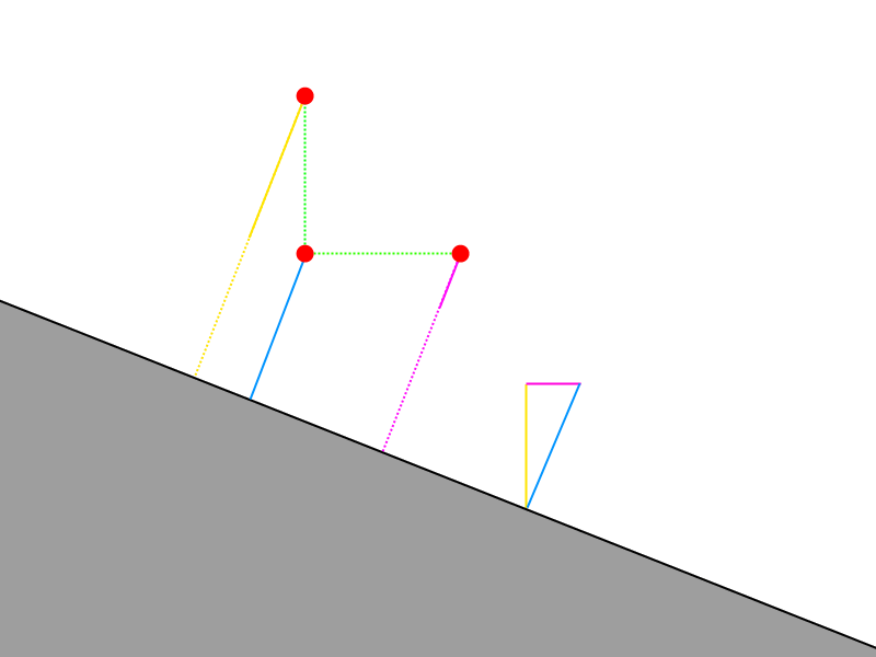
Constructing a perpendicular vector, using the remaining portions of the distance values.

It's important to note that this vector is merely perpendicular to the surface. It still needs to be normalized to be considered a normal vector.

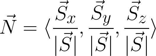
For those who like this kind of thing, here's a pretty LaTeX representation.

Where S is the perpendicular vector, d is the distance function, epsilon is the sampling distance, p is the original point, and N is the surface normal.

An interesting facet of this technique is the fact that we sample distances to surface points that are not that of the original. This requires that the region being sampled has negligible change in gradient for accurate results. Therefore, if epsilon were large enough to span a significant change in slope, the results of this technique would be garbled.

Epsilon, or the maximum acceptable distance, is always linked to the accuracy of spacial representation. This technique then, with its above downfall, additionally ties epsilon's precision with the accuracy of scene lighting and any other effect that relies upon accurate surface orientation.

Something else to think about: What if the original distance was 0.0, and our original point actually did exist upon the geometry? What if the gradient between sample positions was guaranteed to be linear, or at least guaranteed to be safe to assume so? What if we were using traditional rendering techniques, and were working with real fragments with access to dfdx() and dfdy()? What if?