Normally Sampled Ambient Occlusion

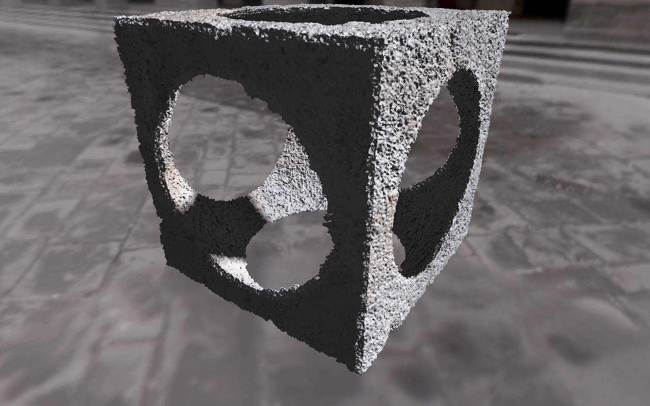
This technique in action in a ray-marched scene. The effect produced is most noticeable in the shadows on the inside of the figure.On my x200 with integrated graphics this runs at 18 fps at 512x312.

The Algorithm

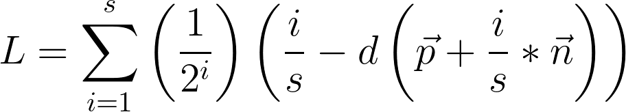
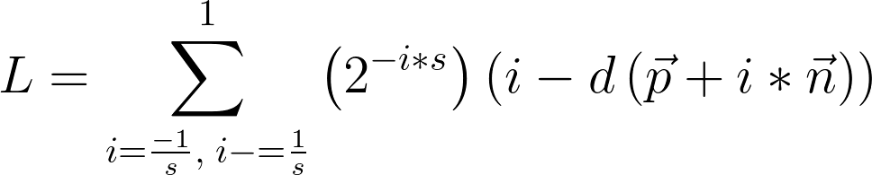
I first learned this technique from a presentation by Inigo Quilez (though that original presentation is nowhere to be found, it seems.) It works by comparing the nearest distance to the surface at points along the surface normal with the point's length along the normal, and using those values as contributions to a sum of how much light was occluded. Let's take a peek, shall we?

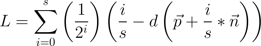
Where L is the amount of occluded light, s is the number of occlusion samples, d is the distance function, p is the surface point, and n is the surface normal.

This is a mean looking equation, so let's break it down. The first thing to note is that the negative exponential out front is to scale samples' contributions to the result by their distance from the surface (or rather their relevance). The subtraction is the comparison between normal distance and sampled distance.

The furthest a point can be from a surface in this situation is its length along the surface normal beneath it. This is important; if the nearest distance is less than this normal distance, then some feature besides the origin surface is near the point. If we assume that this surface is any form opaque, then it is occluding light. This behavior is modelled by the distance function comparison.

However, the greater the length along the surface normal, the greater gap for light to enter. Therefore the contribution of outer samples should be attenuated to suit. The negative power facilitates this.

Illustration

A distance-field terrain with a red sample point and blue normal vector.

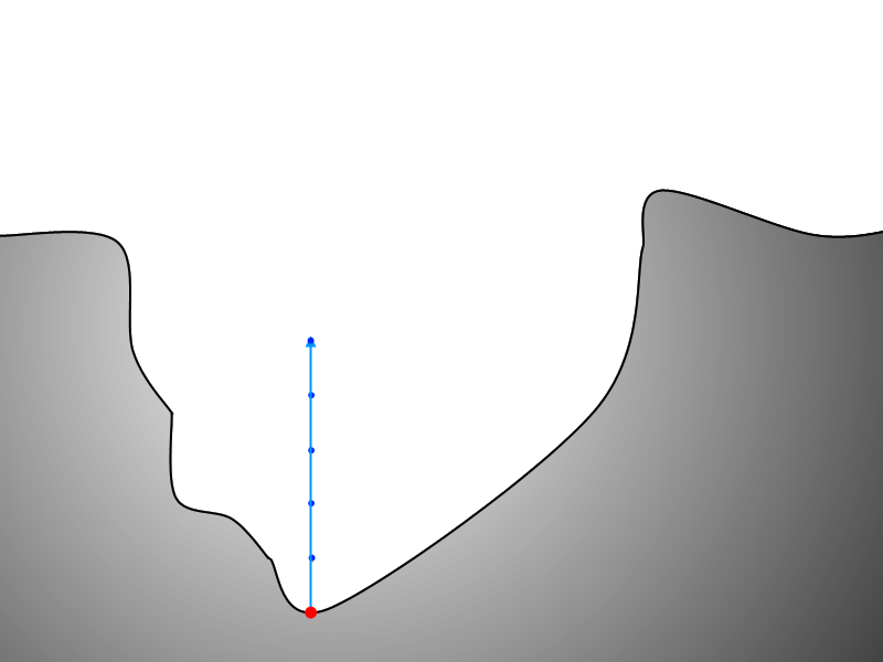
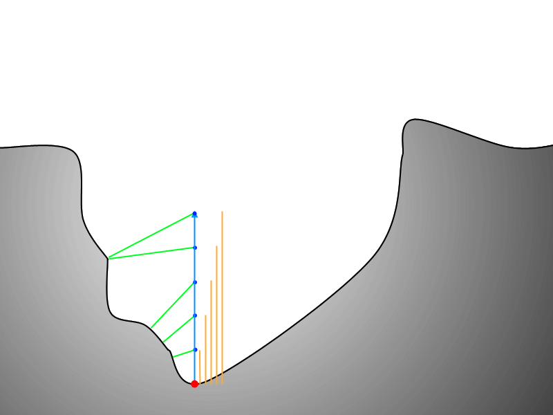
Here we see a basic ray-marched surface with a sample point and normal vector. Next we visualize several discrete steps along this vector.

The surface normal is now divided.

Now that it's established that we discretely step along the normal vector, let's examine exactly why. The figure below highlights the distance along the normal of each surface point.

The surface normal is now divided.

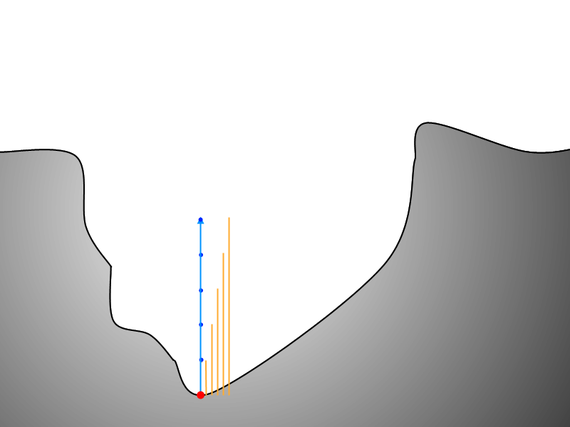
This next figure illustrates the algorithm's depth query.

Depth queries.

Optimization

This technique, as written in the equation above, works well. But there's room to do it much faster. Let's take out a few operations.

Removing the first iteration.

At the first iteration (i=0) the distance along the normal is zero, and the distance to the nearest surface from the original marched point idealistically is also 0. This means that the first contribution is always 0-0, and can be removed.

Removing i/s

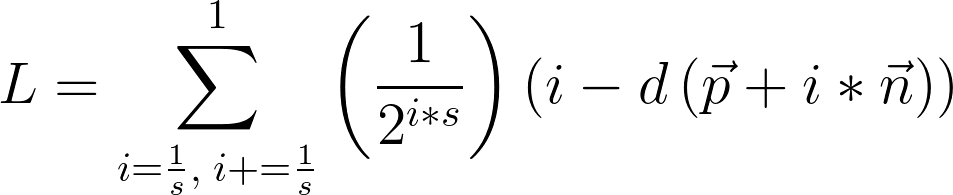
Traditionally the surface normal is of length 1. This assumption is used here, and the length along the normal is considered simply to be the iteration i over the total number of iterations. However, that's a divide for a value that will always range from just above 0 to 1. That means we can pull out those divides and simply update our maximum value and iteration step.

Removing the scaling divide.

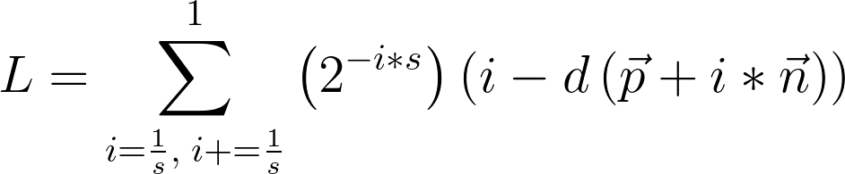
This step is rather obvious. To remove the division in the scale exponential, we negate the power.

Removing the power negation.

As a final touch, we consider s now to be a negative number, and reverse our units, so we don't perform a negation in the scale factor.

Implementation

/*
  Calculates the ambient occlusion factor at a given point in space.
  Uses IQ's marched normal distance comparison technique.
*/
float calcOcclusion(vec3 pos, vec3 norm)
{
  float result = 1.0;
  float s = -OCC_SAMPLES;
  const float unit = 1.0/OCC_SAMPLES;
  for(float i = unit; i < 1.0; i+=unit)
  {
    result -= pow(2.0,i*s)*(i-getDist(pos+i*norm));
  }
  return result*OCC_FACTOR;
}

In implementating this function I found several changes I could make to simplify its contribution to the entire lighting equation.

First, if I subtract each contribution down from 1.0 I can use the resultant value to scale the lighting result, simplifying later stages of my process.

Another implementation difference is that I create a local variable for s. This way I can still specify a positive sample amount, and also no longer need to worry about zany incrementation.

Another facet that differs in the implementation is a final scale factor. This factor was present in the original implementation, but I left it out of my equations to avoid muddling the idea. This is used to scale the appearance of the effect based on how much omni-directional light is in the scene.